How to Embed htmlwidgets into Documents in R

HTML widgets in R Programming Launagauge are interactive web components, JavaScript-based visualizations that can be easily integrated into different documents. They are built on top of the HTML widgets package, which provides a framework for creating R bindings to JavaScript libraries. Examples of HTML widgets available for R include leaflet, dygraphs, Plotly, DiagrammeR, and others.

HTML widgets can be embedded directly into various types of documents created in R, such as R Markdown files, Shiny web applications, and standalone HTML pages, and even indirectly into documents like Word, Excel, PowerPoint, and PDF files. Embedding HTML widgets into documents ensures reproducibility, eliminating any discrepancies that may arise from the manual re-creation of the same document on different setups and environments.

Prerequisites :-

Basics of R programming, HTML widgets in R

The various implementations in different documents have been described below.

1. Standalone HTML Pages

We can embed HTML widgets in standalone HTML pages using the saveWidget() function. This will create an HTML file that includes the necessary JavaScript and CSS dependencies. We can then include the generated HTML file in our HTML document using an iframe tag.

Assume we create a simple HTML widget using Plotly, a popular visualization library. We will create a plot using a preloaded dataset in R. To get a list of preloaded datasets in R type the following in the R console:-

data()

We will use the Morley dataset for our plot, it contains 100 observations where 5 experiments were conducted with 20 observations each for measuring the speed of light. It contains 3 columns `Expt`, `Run`, and `Speed`. We will try to plot a simple line plot with `Run` on the x-axis and `Speed` on the y-axis for 5 different experiments with different colors and save it in a html file named widget.html.

Output:-

001    1   1   850
002    1   2   740
003    1   3   900
004    1   4  1070
005    1   5   930

Output:

htmlwidgets documentation in R

In our plotly widget, the color parameter is passed the factor() passed data structure, here we pass the `Expt` column meaning that with a passed value of the experiment the color of our line plot changes, `mode = “line”` indicates a line plot to be generated.

‘%>% ‘ is the pipe operator which is used to chain multiple function calls together by taking output from the previous function call and passing it as the first argument to the next function call. It allows for a more concise and readable code structure.

After having defined the widget we need to save it as an HTML file using the save widget () function. It contains the following parameters:-

• `widget` is the name of the HTML widget object that we want to save.
• file parameter specifies the name of the file where our widget will be saved.
• selfcontained parameter specifies whether to include all the necessary JavaScript and CSS dependencies within the HTML file itself or not. When self-contained is set to TRUE, the resulting HTML file will be self-contained and can be opened and viewed without any external dependencies.
  

Wait for the code to execute completely, after it finishes notice that the widget.html file is generated in the present working directory. Now open it in the browser to view it.
let’s

2. Shiny application

Shiny is an R package that allows us to build interactive web applications directly from R. In Order to create a simple shiny app we need to have an `app.R` file that contains ui and server. The UI (User Interface) controls the looks and experience of the user and the server function defines the server logic of the Shiny app which controls what is being rendered in the application screen. To install it, type in R console the following:-

install.packages("shiny")

Output:

HTML widget using shiny in R

the

Note :- We can embed more than one html widget into a single document. Please save the above file as ‘app.r’ or ‘app.R‘.

In the above code, we have used an extra library DT which helps in creating interactive tables in HTML. We have used the data table () function of the DT library to convert the wind dataset provided by the Plotly package in R(it is not a preloaded dataset in R) to an interactive HTML table. The package name the

• The UI code above creates a Shiny app layout with two columns. The left column will display the widget1 plot using the plotlyOutput() function and the right column will display the widget2 data table using the dataTableOutput() function from the DT package.
  • fluidPage() function creates a Shiny app UI layout with a fluid design that adjusts to the size of the browser window.
  • fluidRow() function creates a row within the UI layout. It is used to organize the elements horizontally.
  • The column() function creates a column within a row. It is used to allocate space for the UI elements horizontally. We have specified each column a width of 6, which means each widget will occupy the same amount of space within the row.

• In the server() function the `input` parameter receives user interactions in the app and the app performs reactive operations based on them. The `output` parameter represents the output elements i.e. the widgets that are rendered in the UI.
  • output$widget1 binds the output element with the ID “widget1” to the reactive expression { widget1 } using renderPlotly(). The reactive expression will return the value of widget1 when accessed.
  • output$widget2 is similar to above and binds the output element with the ID “widget2” to a reactive expression { widget2 } using renderDataTable() and returns the value of widget2 when accessed.

• shinyApp() function creates the Shiny application object by combining the user interface and server logic allowing us to run and interact with the app.

3. R Markdown Document

R Markdown is a format for creating dynamic documents combining code, text, and visualizations. It is similar to IPython Notebooks in Python programming language though not exactly the same. R Markdown documents are rendered to HTML output by default since it allows for the inclusion of dynamic content like executing code, interactive visualization, and others that are best supported in HTML format.

Output:

R markdown plot

R markdown plot

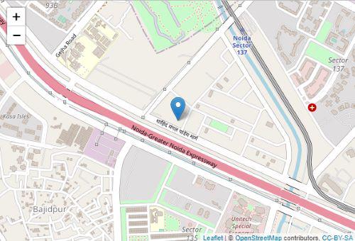
In Widget 1

We have used the leaflet library for interactive maps and marked the GeeksForGeeks office location which initially we saved as coordinates in an array office_loc. Here is the code:-

• addTiles() function adds the default tile layer made by Google Maps to the leaflet widget forming the base of the map.
• addMarkers() function adds a marker to the map in the leaflet widget by taking in parameters lng (longitude), lat (latitude), and popup (text displayed when the marker is clicked). Array indexing in R starts from 1 hence we have accordingly set the latitude and longitude in the addMarkers() function.

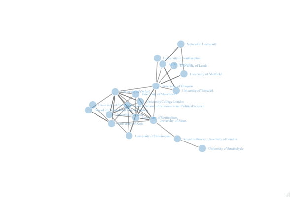
In Widget 2

We have used the networkD3 library to create a simple network graph from R using the dataset SchoolsJournals present in the networkD3 library (It is not a preloaded dataset in R). In the code `seq(100,200,by=2)` all the 51 rows numbered from 100 to 200 skipping two rows in the middle are mentioned in the dataset to be used to create the network graph. The zoom parameter has been set to true so that the graph can be zoomed in and out for clarity. The simple network () function creates our graph after passing the dataset.

4. Word, PowerPoint, Excel, and PDF

Word, PowerPoint, Excel, and PDF are non-HTML formats, hence they do not support the rendering of interactive elements like HTML widgets. To overcome this limitation, we can take a screenshot of the HTML widget and insert the screenshot in the document and thus indirectly embedding the static capture of the widget.

Webshot library in R helps to take screenshots of web pages automating the process of capturing the screenshot after the widget is created rather than us manually capturing screenshots. Before using the webshot package, we need to install it in our R environment. Additionally, the phantomjs tool, which is required by webshot, also needs to be installed.

install.packages("webshot")
webshot::install_phantomjs()

Capturing Screenshots of HTML Output in R Code

First, we will create the HTML widget, then save it as an HTML file and then take a screenshot using the webshop package.

Output:

Plot

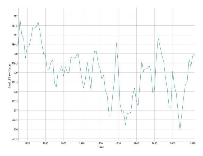
Here we have used the dygraphs package of R. It is used for plotting time-series data i.e. dataset which shows variations with time. There are a couple of preloaded datasets in R to try this out like the EuStockMarkets, austres, JohnsonJohnson, and LakeHuron. Here we will use the LakeHuron dataset which contains data about the levels of Lake Huron from 1875 till 1972.

We simply pass the dataset to the dygraph() function of dygraphs package in order to plot it and for clarity, we have labeled the x-axis as “Time” and the y-axis as “Level of Lake Huron”. The plot generated in the HTML file widget.html is an interactive one. Finally after the a creation of html file the webshot() function takes a screenshot of the widget in the html file as mentioned in url parameter and saves it in the file parameter value.

Capturing Screenshots in the Shiny web application

For capturing screenshots in Shiny web applications, the preferred choice is the shinyscreenshot package instead of webshot. The shinyscreenshot the package is specifically designed as a Shiny extension to offer a simple and convenient solution for capturing screenshots within a Shiny application. It provides an easy way to capture screenshots of specific UI elements or the entire application window.Unlike webshot with PhantomJS, shinyscreenshot does not require any external dependencies or additional installations.

install.packages("shinyscreenshot")

Output:

word cloud
In the above code, we have used the wordcloud2 library to create an interactive word cloud. We have generated a cardioid shape word cloud using the wordcloud2() function with different words present in the demoFreq dataset.

In the UI definition, actionButton() function adds an actionButton widget to the UI for users to click and trigger an action. We have labeled the button as “Take a screenshot” having the ID “go“.

In the server definition, observeEvent() function, the input$go is used to observe changes in the “go” action button. Inside the observer, the screenshot the function is called with the filename parameter set to “screenshot” and the selector parameter ensures only the screenshot of the widget is clicked and not the entire page.

Capturing Screenshots in R Markdown

Output:

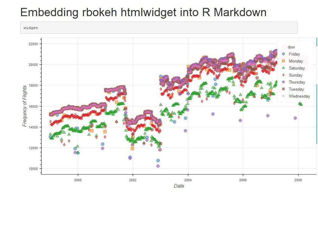
Here we have used the Rbokeh library of R for visualizing the flightfreq dataset that comes with rbokeh library. It contains the frequency of flights in the world from 1999 to 2008. We have tried to plot the date vs frequency of flights and marked all the days of weeks with different colors and different glyphs for more clarity in the plot. In the figure() function, we have specified the parameters of the plot like height width, x-label, and y-label. In the ly_points() function we pass date first as x-axis and then the Freq as the y-axis, the color and glyph parameters for the colorful plot, and the hover parameter controls what to display when we drag the mouse pointer over some point in the plot.

Save it as some “filename.Rmd”, lets assuming filename to be test6.Rmd. No need to render it. Now save the below code in a different R file in the same location.

The rmdshot() function is used to capture screenshots of R Markdown documents. It can handle both static and dynamic R Markdown documents. It first renders the R markdown document and then captures the screenshot. Hence no need to render the R markdown file separately the before compiling above file as it does the operation for us inherently.

After having generated our screenshot we can simply insert the images saved in our personal computer within Word, PowerPoint, Excel or PDF file and do as per requirement.

Inserting screenshot within a Word document

Inserting screenshot within a PowerPoint presentation

joydeep3cq1

Follow

Improve