Last Minute Notes – Operating Systems

An Operating System (OS) is a system software that manages computer hardware, software resources, and provides common services for computer programs. It acts as an interface between the user and the computer hardware.

Types of Operating System (OS):

1. Batch OS – A set of similar jobs are stored in the main memory for execution. A job gets assigned to the CPU, only when the execution of the previous job completes.
2. Multiprogramming OS – The main memory consists of jobs waiting for CPU time. The OS selects one of the processes and assigns it to the CPU. Whenever the executing process needs to wait for any other operation (like I/O), the OS selects another process from the job queue and assigns it to the CPU. This way, the CPU is never kept idle and the user gets the flavor of getting multiple tasks done at once.
   • Multi-Tasking/Time-sharing Operating systems: It is a type of Multiprogramming system with every process running in round robin manner. Each task is given some time to execute so that all the tasks work smoothly. Each user gets the time of the CPU as they use a single system. These systems are also known as Multitasking Systems. The task can be from a single user or different users also. The time that each task gets to execute is called quantum. After this time interval is over OS switches over to the next task.
3. Multi-Processing Operating System: Multi-Processing Operating System is a type of Operating System in which more than one CPU is used for the execution of resources. It betters the throughput of the System.
4. Multi User Operating Systems: These systems allow multiple users to be active at the same time. These system can be either multiprocessor or single processor with interleaving.
5. Distributed Operating System: These types of operating system is a recent advancement in the world of computer technology and are being widely accepted all over the world and, that too, at a great pace. Various autonomous interconnected computers communicate with each other using a shared communication network. Independent systems possess their own memory unit and CPU.
6. Network Operating System: These systems run on a server and provide the capability to manage data, users, groups, security, applications, and other networking functions. These types of operating systems allow shared access to files, printers, security, applications, and other networking functions over a small private network.
7. Real Time OS – Real-Time OS are usually built for dedicated systems to accomplish a specific set of tasks within deadlines.

Threads

A thread is a lightweight process and forms the basic unit of CPU utilization. A process can perform more than one task at the same time by including multiple threads.

• A thread has its own program counter, register set, and stack
• A thread shares resources with other threads of the same process the code section, the data section, files and signals.

A new thread, or a child process of a given process, can be introduced by using the fork() system call.

A process with n fork() system calls generates 2ⁿ – 1 child processes.

There are two types of threads:

• User threads
• Kernel threads

Example: Java thread, POSIX threads. Example : Window Solaris.

Types of Threads

1. Based on the number of threads

There are two types of threads:

(i) Single thread process
(ii) Multi thread process

2. Based on level

There are two types of threads:

(i) User-level threads
(ii) Kernel-level threads

read more about – Threads

Process

A process is a program under execution. The value of program counter (PC) indicates the address of the next instruction of the process being executed. Each process is represented by a Process Control Block (PCB).

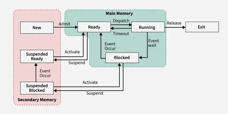
Process States Diagram:

Schedulers

The operating system deploys three kinds of schedulers:

• Long-term scheduler: It is responsible for the creation and bringing of new processes into the main memory (New → Ready state transition).
• Medium-term scheduler: The medium-term scheduler acts as the swapper by doing swap-out (suspending the process from the main to secondary memory) and swap-in (resuming the process by bringing it from the secondary to main memory) operations.
• Short-term scheduler: The short-term scheduler selects a process from the ready state to be executed (Ready → Run state transition).

Dispatchers

The dispatcher is responsible for loading the job (selected by the short-term scheduler) onto the CPU. It performs context switching. Context switching refers to saving the context of the process which was being executed by the CPU and loading the context of the new process that is being scheduled to be executed by the CPU.

CPU Scheduling Algorithms

Why do we need scheduling? A typical process involves both I/O time and CPU time. In a uniprogramming system like MS-DOS, time spent waiting for I/O is wasted and CPU is free during this time. In multiprogramming systems, one process can use CPU while another is waiting for I/O. This is possible only with process scheduling.

Process Scheduling: Below are different times with respect to a process.

• Arrival Time – Time at which the process arrives in the ready queue.
• Completion Time – Time at which process completes its execution.
• Burst Time – Time required by a process for CPU execution.
• Turn Around Time – Time Difference between completion time and arrival time.

Turn Around Time = Completion Time – Arrival Time

• Waiting Time (WT) – Time Difference between turn around time and burst time.

Waiting Time = Turn Around Time – Burst Time

Objectives of Process Scheduling Algorithm:

• Max CPU utilization (Keep CPU as busy as possible)
• Fair allocation of CPU.
• Max throughput (Number of processes that complete their execution per time unit)
• Min turnaround time (Time taken by a process to finish execution)
• Min waiting time (Time for which a process waits in ready queue)
• Min response time (Time when a process produces first response)

Different CPU Scheduling Algorithms:

1. First Come First Serve (FCFS): First Come, First Serve (FCFS) is one of the simplest types of CPU scheduling algorithms. It is exactly what it sounds like: processes are attended to in the order in which they arrive in the ready queue, much like customers lining up at a grocery store.

• It is a non pre-emptive algorithm.
• Processes are assigned to the CPU based on their arrival times. If two or more processes have the same arrival times, then the processes are assigned based on their process ids.
• It is free from starvation

2. Shortest Job First (SJF): Shortest Job First (SJF) or Shortest Job Next (SJN) is a scheduling process that selects the waiting process with the smallest execution time to execute next.

• It is a non-pre-emptive algorithm.
• If all the processes have the same burst times, SJF behaves as FCFS.
• In SJF, the burst times of all the processes should be known prior execution.
• It minimizes the average response time of the processes.
• There is a chance of starvation.

3. Shortest Remaining Time First (SRTF): It is preemptive mode of SJF algorithm in which jobs are scheduled according to the shortest remaining time.

• It is a pre-emptive algorithm.
• Processes are assigned to the CPU based on their shortest remaining burst times.
• If all the processes have the same arrival times, SRTF behaves as SJF.
• It minimizes the average turnaround time of the processes.
• If shorter processes keep on arriving, then the longer processes may starve.

4. Round Robin (RR) Scheduling: It is a method used by operating systems to manage the execution time of multiple processes that are competing for CPU attention.

• RR scheduling is a pre-emptive FCFS based on the concept of time quantum or time slice.
• If the time quantum is too small, then the number of context switches (overhead) will increase and the average response time will decrease.
• If the time quantum is too large, then the number of context switches (overhead) will decrease and the average response time will increase.
• If the time quantum is greater than the burst times of all the processes, RR scheduling behaves as FCFS.

5. Priority Based scheduling: In this scheduling, processes are scheduled according to their priorities, i.e., highest priority process is schedule first. If priorities of two processes match, then scheduling is according to the arrival time.

• Priority scheduling can either be pre-emptive or non-pre-emptive.
• In pre-emptive priority scheduling, a process is voluntarily pre-empted whenever a higher priority process arrives.
• In non-pre-emptive priority scheduling, the scheduler picks up the highest priority process.
• If all the processes have equal priority, then priority scheduling behaves as FCFS.

6. Highest Response Ratio Next (HRRN): In this scheduling, processes with highest response ratio is scheduled. This algorithm avoids starvation.

• It is a non pre-emptive algorithm.
• Processes are assigned to the CPU based on their highest response ratio.
• Response ratio is calculated as:

[Tex]\text{Response Ratio} = \frac{\text{WT} + \text{BT}}{\text{BT}}[/Tex]

• It is free from starvation.
• It favors the shorter jobs and limits the waiting time of the longer jobs.

Some useful facts about Scheduling Algorithms:

1. FCFS can cause long waiting times, especially when the first job takes too much CPU time.
2. Both SJF and Shortest Remaining time first algorithms may cause starvation. Consider a situation when a long process is there in the ready queue and shorter processes keep coming.
3. If time quantum for Round Robin scheduling is very large, then it behaves same as FCFS scheduling.
4. SJF is optimal in terms of average waiting time for a given set of processes. SJF gives minimum average waiting time, but problems with SJF is how to know/predict the time of next job.

read more about – CPU Scheduling Algorithms

Critical Section Problem

1. Critical Section – The portion of the code in the program where shared variables are accessed and/or updated.
2. Remainder Section – The remaining portion of the program excluding the Critical Section.
3. Race around Condition – The final output of the code depends on the order in which the variables are accessed. This is termed as the race around condition.

A solution for the critical section problem must satisfy the following three conditions:

1. Mutual Exclusion – If a process Pi is executing in its critical section, then no other process is allowed to enter into the critical section.
2. Progress – If no process is executing in the critical section, then the decision of a process to enter a critical section cannot be made by any other process that is executing in its remainder section. The selection of the process cannot be postponed indefinitely.
3. Bounded Waiting – There exists a bound on the number of times other processes can enter into the critical section after a process has made request to access the critical section and before the requested is granted.

Synchronization Tools: A Semaphore is an integer variable that is accessed only through two atomic operations, wait () and signal (). An atomic operation is executed in a single CPU time slice without any pre-emption. Semaphores are of two types:

1. Counting Semaphore – A counting semaphore is an integer variable whose value can range over an unrestricted domain.
2. Mutex – A mutex provides mutual exclusion, either producer or consumer can have the key (mutex) and proceed with their work. As long as the buffer is filled by producer, the consumer needs to wait, and vice versa. At any point of time, only one thread can work with the entire buffer. The concept can be generalized using semaphore.
   Misconception: There is an ambiguity between binary semaphore and mutex. We might have come across that a mutex is binary semaphore. But they are not! The purpose of mutex and semaphore are different. May be, due to similarity in their implementation a mutex would be referred as binary semaphore.

read more about – Critical Section Problem

Deadlock

A situation where a set of processes are blocked because each process is holding a resource and waiting for another resource acquired by some other process. Deadlock can arise if following four conditions hold simultaneously (Necessary Conditions):

• Mutual Exclusion – One or more than one resource are non-sharable (Only one process can use at a time).
• Hold and Wait – A process is holding at least one resource and waiting for resources.
• No Preemption – A resource cannot be taken from a process unless the process releases the resource.
• Circular Wait – A set of processes are waiting for each other in circular form.

Deadlock handling

There are three ways to handle deadlock

1. Deadlock prevention

To ensure the system never enters a deadlock state, at least one of the conditions for deadlock must be prevented:

• Mutual Exclusion: This condition cannot be removed because some resources (non-shareable resources) must be exclusively allocated to one process at a time.
• Hold and Wait: This condition can be avoided using the following strategies:
  • Allocate all required resources to a process before it starts execution. However, this approach might lead to low resource utilization.
  • Force a process to release all its held resources before requesting new ones. However, this might cause starvation (a process waiting indefinitely).
• Pre-emption:
  • If a process P1P1P1 requests a resource RRR that is held by another process P2P2P2:
    • If P2P2P2 is still running, P1P1P1 will have to wait.
    • Otherwise, the resource RRR can be taken (pre-empted) from P2P2P2 and allocated to P1P1P1.
• Circular Wait: This condition can be avoided using the following method:
  • Assign a unique number to each resource (assuming there is only one instance of each resource).
  • Ensure processes request resources in a strict order, either increasing or decreasing based on the assigned numbers.

2. Deadlock Avoidance

The Deadlock Avoidance Algorithm prevents deadlocks by monitoring resource usage and resolving conflicts before they occur, like rolling back processes or reallocating resources. It minimizes deadlocks but doesn’t fully guarantee their prevention. The two key techniques are:

1. Process Initiation Denial: Blocks processes that might cause deadlock.
2. Resource Allocation Denial: Rejects resource requests that could lead to deadlock.

Banker’s Algorithm

The Banker’s Algorithm is a resource allocation and deadlock avoidance algorithm used in operating systems. It ensures that the system remains in a safe state by simulating the allocation of resources to processes without running into a deadlock.

The following Data structures are used to implement the Banker’s Algorithm:

1. Available: It is a 1-D array of size ‘m’ indicating the number of available resources of each type. Available[ j ] = k means there are ‘k’ instances of resource type R _j.

2. Max: It is a 2-d array of size ‘ n*m’ that defines the maximum demand of each process in a system. Max[ i, j ] = k means process P_i may request at most ‘k’ instances of resource type R_j.

3.Allocated: It is a 2-d array of size ‘n*m’ that defines the number of resources of each type currently allocated to each process. Allocation[ i, j ] = k means process P_i is currently allocated ‘k’ instances of resource type R_j.

4. Need: It is a 2-d array of size ‘n*m’ that indicates the remaining resource need of each process. Need [ i,   j ] = k means process P_i currently needs ‘k’ instances of resource type R_j Need [ i,   j ] = Max [ i,   j ] – Allocation [ i,   j ].

3. Deadlock Detection and Recovery

Detection: A cycle in the resource allocation graph represents deadlock only when resources are of single-instance type. If the resources are of multiple instance type, then the safety algorithm is used to detect deadlock.

Recovery: A system can recover from deadlock through adoption of the following mechanisms:

• Process termination
• Resource Pre-emption

4. Deadlock Ignorance

In the Deadlock ignorance method the OS acts like the deadlock never occurs and completely ignores it even if the deadlock occurs. This method only applies if the deadlock occurs very rarely. The algorithm is very simple. It says, ” if the deadlock occurs, simply reboot the system and act like the deadlock never occurred.” That’s why the algorithm is called the Ostrich Algorithm. 

read more about – Deadlock

Memory Management

In multiprogramming system, the task of subdividing the memory among the various processes is called memory management. The task of the memory management unit is the efficient utilization of memory and minimize the internal and external fragmentation.

Why Memory Management is Required?

• Allocate and de-allocate memory before and after process execution.
• To keep track of used memory space by processes.
• To minimize fragmentation issues.
• To proper utilization of main memory.
• To maintain data integrity while executing of process.

Logical and Physical Address Space

• Logical Address Space: An address generated by the CPU is known as a “Logical Address”. It is also known as a Virtual address. Logical address space can be defined as the size of the process. A logical address can be changed.

• Physical Address Space: An address seen by the memory unit (i.e. the one loaded into the memory address register of the memory) is commonly known as a “Physical Address”. A Physical address is also known as a Real address.

Static and Dynamic Loading

Loading a process into the main memory is done by a loader. There are two different types of loading :

• Static Loading: Static Loading is basically loading the entire program into a fixed address. It requires more memory space.

• Dynamic Loading: The entire program and all data of a process must be in physical memory for the process to execute. So, the size of a process is limited to the size of physical memory. To gain proper memory utilization, dynamic loading is used. In dynamic loading, a routine is not loaded until it is called.

Memory Management Techniques

(a) Single Partition Allocation Schemes – The memory is divided into two parts. One part is kept to be used by the OS and the other is kept to be used by the users.
(b) Multiple Partition Schemes –

1. Fixed Partition – The memory is divided into fixed size partitions.
2. Variable Partition – The memory is divided into variable sized partitions.

Variable partition allocation schemes:

1. First Fit – The arriving process is allotted the first hole of memory in which it fits completely.
2. Best Fit – The arriving process is allotted the hole of memory in which it fits the best by leaving the minimum memory empty.
3. Worst Fit – The arriving process is allotted the hole of memory in which it leaves the maximum gap.

Note:

• Best fit does not necessarily give the best results for memory allocation.
• The cause of external fragmentation is the condition in Fixed partitioning and Variable partitioning saying that entire process should be allocated in a contiguous memory location. Therefore Paging is used.

Paging

The physical memory is divided into equal sized frames. The main memory is divided into fixed size pages. The size of a physical memory frame is equal to the size of a virtual memory frame.

Segmentation

Segmentation is implemented to give users view of memory. The logical address space is a collection of segments. Segmentation can be implemented with or without the use of paging.

read more about – Memory Management Techniques

Page Fault: A page fault is a type of interrupt, raised by the hardware when a running program accesses a memory page that is mapped into the virtual address space, but not loaded in main/virtual memory.

Page Replacement Algorithms

1. First In First Out (FIFO)

This is the simplest page replacement algorithm. In this algorithm, operating system keeps track of all pages in the memory in a queue, oldest page is in the front of the queue. When a page needs to be replaced page in the front of the queue is selected for removal.

For example, consider page reference string 1, 3, 0, 3, 5, 6 and 3 page slots.

• Initially, all slots are empty, so when 1, 3, 0 came they are allocated to the empty slots —> 3 Page Faults.
• When 3 comes, it is already in memory so —> 0 Page Faults. Then 5 comes, it is not available in memory so it replaces the oldest page slot i.e 1. —> 1 Page Fault.
• Finally, 6 comes,  it is also not available in memory so it replaces the oldest page slot i.e 3 —> 6 Page Fault.

Belady’s anomaly: Belady’s anomaly proves that it is possible to have more page faults when increasing the number of page frames while using the First in First Out (FIFO) page replacement algorithm. 

For example, if we consider reference string      3     2     1     0     3     2     4     3     2     1     0     4 and 3 slots, we get 9 total page faults, but if we increase slots to 4, we get 10 page faults.

2. Optimal Page replacement

In this algorithm, pages are replaced which are not used for the longest duration of time in the future.

Let us consider page reference string 7 0 1 2 0 3 0 4 2 3 0 3 2 and 4 page slots.

Initially, all slots are empty, so when 7 0 1 2 are allocated to the empty slots —> 4 Page faults.
0 is already there so —> 0 Page fault.
When 3 came it will take the place of 7 because it is not used for the longest duration of time in the future.—> 1 Page fault.
0 is already there so —> 0 Page fault.
4 will takes place of 1 —> 1 Page Fault.
Now for the further page reference string —> 0 Page fault because they are already available in the memory.

Optimal page replacement is perfect, but not possible in practice as an operating system cannot know future requests. The use of Optimal Page replacement is to set up a benchmark so that other replacement algorithms can be analyzed against it.

3. Least Recently Used (LRU)

In this algorithm, the page will be replaced which is least recently used.

Let say the page reference string 7 0 1 2 0 3 0 4 2 3 0 3 2 .

Initially, we have 4-page slots empty. Initially, all slots are empty, so when 7 0 1 2 are allocated to the empty slots —> 4 Page faults.
0 is already their so —> 0 Page fault.
When 3 came it will take the place of 7 because it is least recently used —> 1 Page fault.
0 is already in memory so —> 0 Page fault. 4 will takes place of 1 —> 1 Page Fault.
Now for the further page reference string —> 0 Page fault because they are already available in the memory.

4. Most Recently Used (MRU)

In this algorithm, page will be replaced which has been used recently. Belady’s anomaly can occur in this algorithm.

Example: Consider the page reference string 7, 0, 1, 2, 0, 3, 0, 4, 2, 3, 0, 3, 2, 3 with 4-page frames. Find number of page faults using MRU Page Replacement Algorithm.

• Initially, all slots are empty, so when 7 0 1 2 are allocated to the empty slots —> 4 Page faults
• 0 is already their so–> 0 page fault
• when 3 comes it will take place of 0 because it is most recently used —> 1 Page fault
• when 0 comes it will take place of 3  —> 1 Page fault
• when 4 comes it will take place of 0  —> 1 Page fault
• 2 is already in memory so —> 0 Page fault
• when 3 comes it will take place of 2  —> 1 Page fault
• when 0 comes it will take place of 3  —> 1 Page fault
• when 3 comes it will take place of 0  —> 1 Page fault
• when 2 comes it will take place of 3  —> 1 Page fault
• when 3 comes it will take place of 2  —> 1 Page fault

read more about – Page Replacement Algorithms

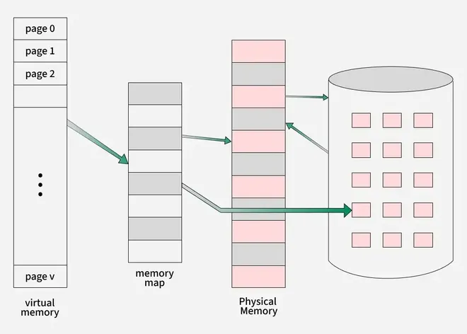
Virtual Memory

Virtual memory is a memory management technique used by operating systems to give the appearance of a large, continuous block of memory to applications, even if the physical memory (RAM) is limited. It allows larger applications to run on systems with less RAM.

Demand Paging

Demand paging is a memory management technique used in operating systems where a page (a fixed-size block of memory) is only loaded into the computer’s RAM when it is needed, or “demanded” by a process.

How Demand Paging Works:

1. When a Program Starts: Initially, only a part of the program (some pages) is loaded into RAM. The rest of the program is stored on the hard drive (secondary memory).
2. When a Page is Needed: If the program needs a page that is not currently in RAM, a page fault occurs. This means the operating system must fetch the required page from the hard drive and load it into RAM.
3. Efficient Memory Use: With demand paging, only the parts of the program that are actively used are in memory, which makes better use of RAM. This allows the system to run large programs without needing all of their data loaded into memory at once.

read more about – Demand Paging

Thrashing

Thrashing is a situation in which the operating system spends more time swapping data between RAM (main memory) and the hard drive (secondary memory) than actually executing processes. This happens when there isn’t enough physical memory (RAM) to handle the current workload, causing the system to constantly swap pages in and out of memory.

Techniques to handle Thrashing

read more about – Virtual Memory

File Systems

A file system is a method an operating system uses to store, organize, and manage files and directories on a storage device.

File Directories

The collection of files is a file directory. The directory contains information about the files, including attributes, location, and ownership. Much of this information, especially that is concerned with storage, is managed by the operating system.

Below are information contained in a device directory.

• Name
• Type
• Address
• Current length
• Maximum length
• Date last accessed
• Date last updated
• Owner id
• Protection information

The operation performed on the directory are: 

• Search for a file
• Create a file
• Delete a file
• List a directory
• Rename a file
• Traverse the file system

File Allocation Methods

There are several types of file allocation methods. These are mentioned below.

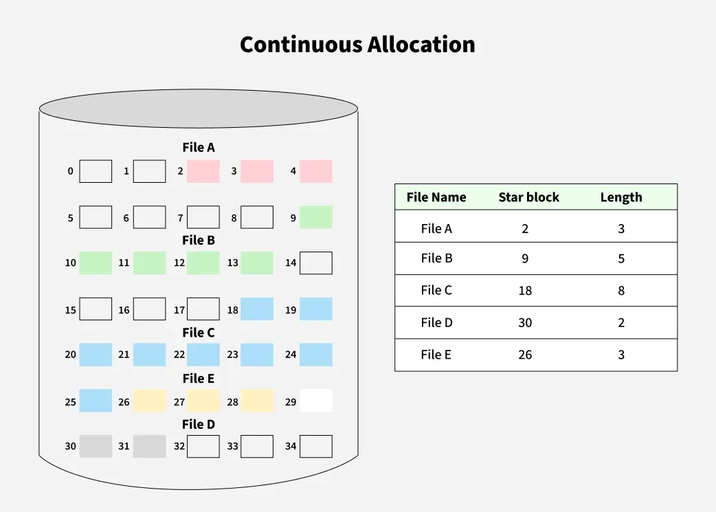
Continuous Allocation: A single continuous set of blocks is allocated to a file at the time of file creation. Thus, this is a pre-allocation strategy, using variable size portions. The file allocation table needs just a single entry for each file, showing the starting block and the length of the file.

Linked Allocation(Non-contiguous allocation): Allocation is on an individual block basis. Each block contains a pointer to the next block in the chain. Again the file table needs just a single entry for each file, showing the starting block and the length of the file. Although pre-allocation is possible, it is more common simply to allocate blocks as needed. Any free block can be added to the chain.

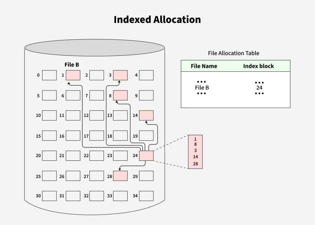
Indexed Allocation: Allocation is on an individual block basis. Each block contains a pointer to the next block in the chain. Again the file table needs just a single entry for each file, showing the starting block and the length of the file. Although pre-allocation is possible, it is more common simply to allocate blocks as needed. Any free block can be added to the chain.

read more about – File Systems

Disk Scheduling

Disk scheduling algorithms are crucial in managing how data is read from and written to a computer’s hard disk. These algorithms help determine the order in which disk read and write requests are processed, significantly impacting the speed and efficiency of data access. Common disk scheduling methods include First-Come, First-Served (FCFS), Shortest Seek Time First (SSTF), SCAN, C-SCAN, LOOK, and C-LOOK. By understanding and implementing these algorithms, we can optimize system performance and ensure faster data retrieval.

Disk scheduling Algorithms

Different Disk scheduling Algorithms are:

• FCFS (First Come First Serve): FCFS is the simplest of all Disk Scheduling Algorithms. In FCFS, the requests are addressed in the order they arrive in the disk queue. 

• SSTF (Shortest Seek Time First): In SSTF (Shortest Seek Time First), requests having the shortest seek time are executed first. So, the seek time of every request is calculated in advance in the queue and then they are scheduled according to their calculated seek time. As a result, the request near the disk arm will get executed first. SSTF is certainly an improvement over FCFS as it decreases the average response time and increases the throughput of the system. 

• SCAN: In the SCAN algorithm the disk arm moves in a particular direction and services the requests coming in its path and after reaching the end of the disk, it reverses its direction and again services the request arriving in its path. So, this algorithm works as an elevator and is hence also known as an elevator algorithm. As a result, the requests at the midrange are serviced more and those arriving behind the disk arm will have to wait.

• C-SCAN: In the SCAN algorithm, the disk arm again scans the path that has been scanned, after reversing its direction. So, it may be possible that too many requests are waiting at the other end or there may be zero or few requests pending at the scanned area.

• LOOK: LOOK Algorithm is similar to the SCAN disk scheduling algorithm except for the difference that the disk arm in spite of going to the end of the disk goes only to the last request to be serviced in front of the head and then reverses its direction from there only. Thus it prevents the extra delay which occurred due to unnecessary traversal to the end of the disk.

• C-LOOK: As LOOK is similar to the SCAN algorithm, in a similar way, C-LOOK is similar to the CSCAN disk scheduling algorithm. In CLOOK, the disk arm in spite of going to the end goes only to the last request to be serviced in front of the head and then from there goes to the other end’s last request. Thus, it also prevents the extra delay which occurred due to unnecessary traversal to the end of the disk.

• LIFO (Last-In First-Out): In LIFO (Last In, First Out) algorithm, the newest jobs are serviced before the existing ones i.e. in order of requests that get serviced the job that is newest or last entered is serviced first, and then the rest in the same order.

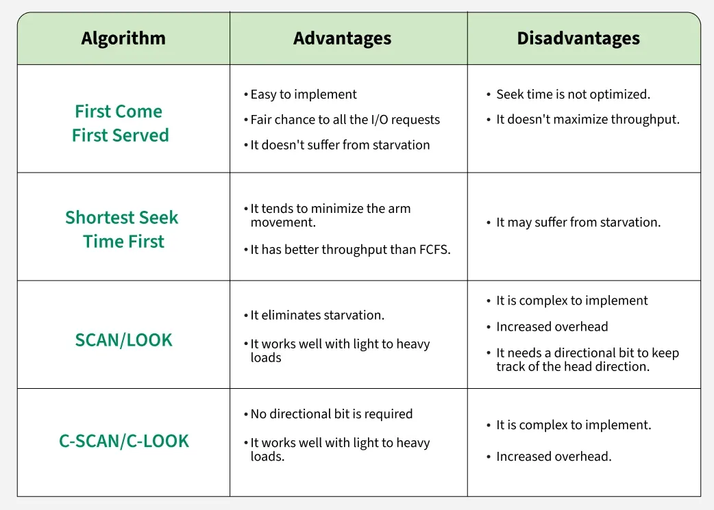
Comparison Among the Disk Scheduling Algorithms

read more about – Disk scheduling algorithms

kartik

Follow

Improve

Article Tags :

• GATE CS
• Operating Systems