What are Graph Neural Networks?
Last Updated :
15 Nov, 2024
Graph Neural Networks (GNNs) are a neural network specifically designed to work with data represented as graphs. Unlike traditional neural networks, which operate on grid-like data structures like images (2D grids) or text (sequential), GNNs can model complex, non-Euclidean relationships in data, such as social networks, molecular structures, and knowledge graphs.
This article explores what GNNs are, how they work, their types, and their wide range of applications.
Understanding Graph Structures
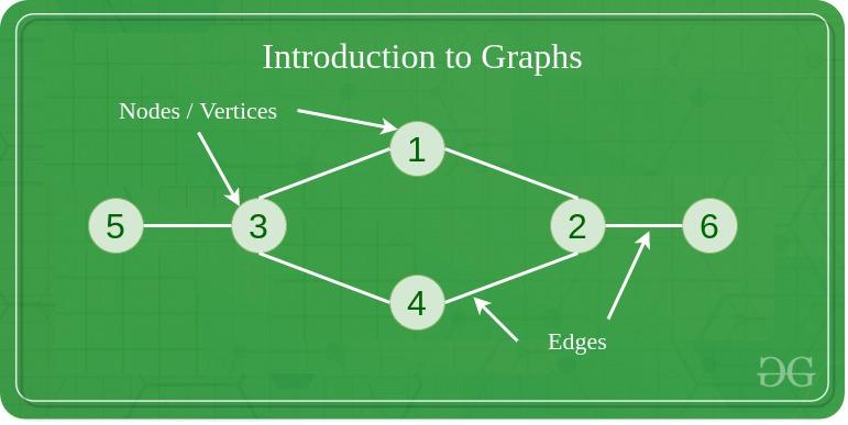
A graph is a data structure that represents relationships between pairs of objects. Each object is known as a node (or vertex), and each connection between nodes is an edge.

Nodes and Vertices in Graph Data Structure
Graphs can vary based on the type of edges:
- Directed Graphs: In these graphs, edges have a direction, indicated by an arrow, showing a one-way relationship from one node to another.
- Undirected Graphs: In these graphs, edges are bidirectional, representing two-way relationships without any direction.
Types of Graphs
Graphs can be classified based on their structural properties:
| Type of Graph | Description | Example/Use Case |
|---|
| Homogeneous Graph | Contains only one type of node and edge, simplifying representation and analysis. | Social network with people as nodes and friendships as edges. |
| Heterogeneous Graph | Consists of multiple types of nodes and edges, suitable for complex relationships. | Knowledge graph with nodes for entities (people, places) and varied edges. |
| Static Graph | Remains fixed once created, with no changes to nodes or edges. | Scenarios where relationships are constant over time. |
| Dynamic Graph | Allows the addition or deletion of nodes and edges, ideal for situations with frequently changing relationships. | Real-time communication tracking or evolving social networks. |
Graph Data Representation
There are multiple ways to represent graph data, each serving different use cases:
- Adjacency Matrix: A square matrix where each cell indicates if an edge exists between two nodes; best for dense graphs.
- Feature Matrices: Stores attributes for nodes and edges, such as age or connection strength, adding context to graph data.
- Adjacency List: Each node lists its neighboring nodes, making it efficient for sparse graphs.
- Edge List: Represents edges as pairs of nodes, useful in algorithms that focus on processing edges directly.
Basics of Graph Neural Networks
Graph Neural Networks (GNNs) are a class of neural networks designed specifically to work with graph-structured data. They’re used to learn patterns and relationships between connected entities within a graph, making them ideal for applications like social networks, recommendation systems, and molecular studies.
How GNNs Process Graph Data?
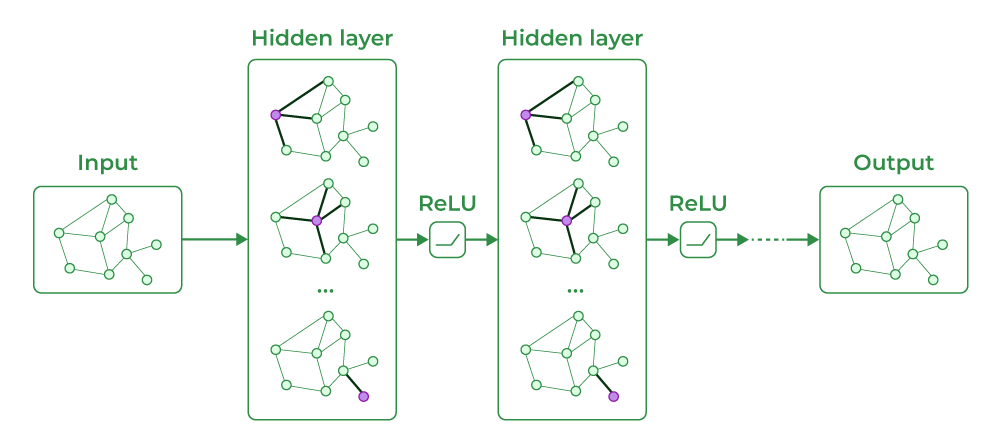
GNNs process graph data by passing information between nodes through their connections (edges). Each node gathers information from its neighbors in a process called message passing, allowing it to learn representations based on its local structure and features. This iterative information-sharing allows nodes to understand the context provided by surrounding nodes in the graph.
Key Concepts of GNNs
- Message Passing: In GNNs, each node aggregates information from its neighbors through a process called “message passing.” The node then updates its representation based on this aggregated information.
- Node Embeddings: The final result of message passing is an embedding or feature vector for each node. These embeddings can capture complex patterns and dependencies in the graph structure.
- Graph-Level Representations: In addition to node embeddings, some GNN architectures can produce representations for the entire graph, making them suitable for graph-level tasks such as graph classification.
How Do Graph Neural Networks Work?
A typical GNN operates in three steps:
- Initialization: Each node is initialized with its feature vector, which could represent properties like age, gender, or molecular weight, depending on the application.
- Message Passing: Over several iterations or “layers,” nodes exchange information with their neighbors, aggregating data from connected nodes.
- Update: Each node updates its feature vector using aggregated information, often by applying a neural network layer (e.g., a linear transformation followed by a non-linear activation function).
Types of Graph Neural Networks (GNNs)
1. Graph Convolutional Networks (GCN)
GCNs extend the concept of convolutional neural networks to graph data. They work by aggregating information from a node’s neighbors to update its representation. This aggregation is done in multiple layers, allowing GCNs to capture both local and global structural information in the graph. GCNs are particularly effective for semi-supervised learning tasks, such as node classification.

Graph Convolutional Networks (GCN)
2. Graph Attention Networks (GAT)
GATs introduce an attention mechanism to GNNs, allowing the model to weigh the importance of neighboring nodes differently during message passing. This adaptive focus helps GATs capture complex relationships and varying influence levels between nodes, improving performance on tasks where certain connections are more significant than others, such as in social networks or citation networks.
3. Graph Recurrent Networks (GRN)
GRNs combine the principles of recurrent neural networks (RNNs) with graph structures. They are designed to handle temporal dynamics in graph data, making them suitable for scenarios where relationships evolve over time. GRNs can effectively model sequences of graph changes, such as social interactions or traffic flow.
4. Spatial and Spectral-based GNNs
- Spatial-based GNNs operate directly on the graph structure, focusing on the spatial relationships between nodes. They leverage the graph topology to propagate information.
- Spectral-based GNNs utilize spectral graph theory, applying techniques from Fourier analysis to define convolutions on graphs. These networks typically operate in the spectral domain, allowing them to capture global properties of the graph.
After multiple layers of message passing, each node’s feature vector (embedding) contains not only its own information but also information about its neighbors and potentially, the whole graph structure.
Implementing Graph Neural Network for Node Classification on the Cora Dataset
Step 1: Install Required Libraries
The first lines install the required libraries for working with PyTorch and PyTorch Geometric.
!pip install torch torchvision torchaudio!pip install torch-geometric
Step 2: Import Libraries
Here, essential libraries are imported, including:
- PyTorch and torch.nn for defining neural networks and optimizing them.
- torch_geometric for graph neural network operations.
- matplotlib and networkx for visualizing graphs.
Python
import torch
import torch.nn as nn
import torch.optim as optim
from torch_geometric.datasets import Planetoid
from torch_geometric.nn import GCNConv
import matplotlib.pyplot as plt
import networkx as nx
Step 3: Define the GCN Model
The Graph Convolutional Network (GCN) model class is defined. The model has two layers:
conv1: A GCN layer taking input features and transforming them to hidden channels.conv2: A GCN layer transforming hidden channels to output classes.
Python
# Define the GCN model
class GCN(nn.Module):
    def __init__(self, in_channels, hidden_channels, out_channels):
        super(GCN, self).__init__()
        self.conv1 = GCNConv(in_channels, hidden_channels)
        self.conv2 = GCNConv(hidden_channels, out_channels)

    def forward(self, x, edge_index):
        x = self.conv1(x, edge_index).relu()
        x = self.conv2(x, edge_index)
        return x
Step 4: Load the Cora Dataset
The Planetoid dataset loader loads the Cora dataset, commonly used for graph learning tasks. The dataset includes the graph structure and node labels.
Python
# Load the Cora dataset
dataset = Planetoid(root='/tmp/Cora', name='Cora')
data = dataset[0]  # Get the first graph object
Step 5: Initialize Model, Optimizer, and Loss Function
An instance of the GCN model is created, along with an optimizer (Adam) and loss function (Cross-Entropy Loss).
Python
# Initialize model, optimizer, and loss function
model = GCN(in_channels=dataset.num_node_features, hidden_channels=16, out_channels=dataset.num_classes)
optimizer = optim.Adam(model.parameters(), lr=0.01)
criterion = nn.CrossEntropyLoss()
Step 6: Define the Training Function
The train function performs a forward pass, calculates the loss, backpropagates the loss, and updates the model’s parameters.
Python
# Training loop
def train():
    model.train()
    optimizer.zero_grad()  # Clear gradients
    out = model(data.x, data.edge_index)  # Forward pass
    loss = criterion(out[data.train_mask], data.y[data.train_mask])  # Compute loss
    loss.backward()  # Backpropagation
    optimizer.step()  # Update weights
    return loss.item()
Step 7: Define the Evaluation Function
The test function evaluates the model on the test set without calculating gradients.
Python
# Evaluation function
def test():
    model.eval()
    with torch.no_grad():  # No gradients needed for evaluation
        out = model(data.x, data.edge_index)
        pred = out.argmax(dim=1)  # Get the predicted classes
        test_accuracy = (pred[data.test_mask] == data.y[data.test_mask]).sum() / data.test_mask.sum()
        return test_accuracy.item()
Step 8: Train the Model
This loop trains the model for 200 epochs and prints the loss and test accuracy every 10 epochs.
Python
# Run the training process
for epoch in range(200):  # Number of epochs
    loss = train()
    if epoch % 10 == 0:
        test_acc = test()
        print(f'Epoch: {epoch}, Loss: {loss:.4f}, Test Accuracy: {test_acc:.4f}')

print("Training completed.")
Output:
Epoch: 0, Loss: 1.9398, Test Accuracy: 0.3830
Epoch: 10, Loss: 0.5945, Test Accuracy: 0.7890
Epoch: 20, Loss: 0.0978, Test Accuracy: 0.7870
.
.
.
Epoch: 180, Loss: 0.0009, Test Accuracy: 0.7870
Epoch: 190, Loss: 0.0008, Test Accuracy: 0.7870
Training completed.
Step 9: Plot an Interactive Graph of the Cora Dataset
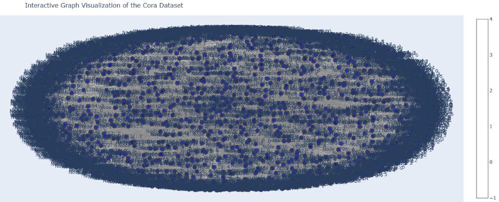
Using NetworkX and Plotly, an interactive graph of the Cora dataset is created with node colors representing different classes.
Python
import numpy as np
import plotly.graph_objs as go
import plotly.offline as pyo
import networkx as nx

# Function to plot the interactive graph
def plot_interactive_graph():
    # Create a NetworkX graph from edge index
    edge_index = data.edge_index.cpu().numpy()  # Convert to NumPy array
    G = nx.Graph()

    # Add edges to the graph
    for i in range(edge_index.shape[1]):
        G.add_edge(edge_index[0, i], edge_index[1, i])

    # Node labels and colors
    labels = {i: dataset[0].y[i].item() for i in range(data.num_nodes)}  # Node labels based on class
    colors = np.array([dataset[0].y[i].item() for i in range(data.num_nodes)])  # Node colors based on class

    # Create position layout for nodes
    pos = nx.spring_layout(G, k=0.5, iterations=50)  # Positioning of nodes

    # Prepare data for Plotly
    edge_x = []
    edge_y = []
    for edge in G.edges():
        x0, y0 = pos[edge[0]]
        x1, y1 = pos[edge[1]]
        edge_x.append(x0)
        edge_x.append(x1)
        edge_x.append(None)  # None to break lines between edges
        edge_y.append(y0)
        edge_y.append(y1)
        edge_y.append(None)  # None to break lines between edges

    edge_trace = go.Scatter(
        x=edge_x, y=edge_y,
        line=dict(width=0.5, color='#888'),
        hoverinfo='none',
        mode='lines'
    )

    node_x = []
    node_y = []
    node_color = []
    for i in range(data.num_nodes):
        x, y = pos[i]
        node_x.append(x)
        node_y.append(y)
        # Generate monochromatic color based on the class
        node_color.append(f'rgba(0, 0, {255 - (colors[i] * 25)}, 0.7)')  # Blue shades based on class

    node_trace = go.Scatter(
        x=node_x, y=node_y,
        mode='markers+text',
        hoverinfo='text',
        marker=dict(showscale=True,
                    colorscale='Blues',
                    size=10,
                    color=node_color,
                    line=dict(width=2)),
        text=[f'Node {i}: {labels[i]}' for i in range(data.num_nodes)]
    )

    # Create the figure
    fig = go.Figure(data=[edge_trace, node_trace],
                    layout=go.Layout(
                        title='Interactive Graph Visualization of the Cora Dataset',
                        titlefont=dict(size=16),
                        showlegend=False,
                        hovermode='closest',
                        margin=dict(b=0,l=0,r=0,t=40),
                        xaxis=dict(showgrid=False, zeroline=False, showticklabels=False),
                        yaxis=dict(showgrid=False, zeroline=False, showticklabels=False)
                    ))

    pyo.iplot(fig)  # Use pyo.plot(fig) if you're using a script outside Jupyter Notebook

# Call the function to plot the interactive graph
plot_interactive_graph()
Output:

Interactive Graph Visualization of the Cora Dataset

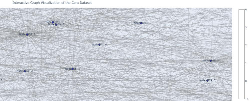
Zoomed Image of the above graph visualization
Complete Code
You can download the source code from here.
Python
import torch
import torch.nn as nn
import torch.optim as optim
from torch_geometric.datasets import Planetoid
from torch_geometric.nn import GCNConv
import matplotlib.pyplot as plt
import networkx as nx

# Define the GCN model
class GCN(nn.Module):
    def __init__(self, in_channels, hidden_channels, out_channels):
        super(GCN, self).__init__()
        self.conv1 = GCNConv(in_channels, hidden_channels)
        self.conv2 = GCNConv(hidden_channels, out_channels)

    def forward(self, x, edge_index):
        x = self.conv1(x, edge_index).relu()
        x = self.conv2(x, edge_index)
        return x

# Load the Cora dataset
dataset = Planetoid(root='/tmp/Cora', name='Cora')
data = dataset[0]  # Get the first graph object

# Initialize model, optimizer, and loss function
model = GCN(in_channels=dataset.num_node_features, hidden_channels=16, out_channels=dataset.num_classes)
optimizer = optim.Adam(model.parameters(), lr=0.01)
criterion = nn.CrossEntropyLoss()

# Training loop
def train():
    model.train()
    optimizer.zero_grad()  # Clear gradients
    out = model(data.x, data.edge_index)  # Forward pass
    loss = criterion(out[data.train_mask], data.y[data.train_mask])  # Compute loss
    loss.backward()  # Backpropagation
    optimizer.step()  # Update weights
    return loss.item()

# Evaluation function
def test():
    model.eval()
    with torch.no_grad():  # No gradients needed for evaluation
        out = model(data.x, data.edge_index)
        pred = out.argmax(dim=1)  # Get the predicted classes
        test_accuracy = (pred[data.test_mask] == data.y[data.test_mask]).sum() / data.test_mask.sum()
        return test_accuracy.item()

# Run the training process
for epoch in range(200):  # Number of epochs
    loss = train()
    if epoch % 10 == 0:
        test_acc = test()
        print(f'Epoch: {epoch}, Loss: {loss:.4f}, Test Accuracy: {test_acc:.4f}')

print("Training completed.")

import numpy as np
import plotly.graph_objs as go
import plotly.offline as pyo
import networkx as nx

# Function to plot the interactive graph
def plot_interactive_graph():
    # Create a NetworkX graph from edge index
    edge_index = data.edge_index.cpu().numpy()  # Convert to NumPy array
    G = nx.Graph()

    # Add edges to the graph
    for i in range(edge_index.shape[1]):
        G.add_edge(edge_index[0, i], edge_index[1, i])

    # Node labels and colors
    labels = {i: dataset[0].y[i].item() for i in range(data.num_nodes)}  # Node labels based on class
    colors = np.array([dataset[0].y[i].item() for i in range(data.num_nodes)])  # Node colors based on class

    # Create position layout for nodes
    pos = nx.spring_layout(G, k=0.5, iterations=50)  # Positioning of nodes

    # Prepare data for Plotly
    edge_x = []
    edge_y = []
    for edge in G.edges():
        x0, y0 = pos[edge[0]]
        x1, y1 = pos[edge[1]]
        edge_x.append(x0)
        edge_x.append(x1)
        edge_x.append(None)  # None to break lines between edges
        edge_y.append(y0)
        edge_y.append(y1)
        edge_y.append(None)  # None to break lines between edges

    edge_trace = go.Scatter(
        x=edge_x, y=edge_y,
        line=dict(width=0.5, color='#888'),
        hoverinfo='none',
        mode='lines'
    )

    node_x = []
    node_y = []
    node_color = []
    for i in range(data.num_nodes):
        x, y = pos[i]
        node_x.append(x)
        node_y.append(y)
        # Generate monochromatic color based on the class
        node_color.append(f'rgba(0, 0, {255 - (colors[i] * 25)}, 0.7)')  # Blue shades based on class

    node_trace = go.Scatter(
        x=node_x, y=node_y,
        mode='markers+text',
        hoverinfo='text',
        marker=dict(showscale=True,
                    colorscale='Blues',
                    size=10,
                    color=node_color,
                    line=dict(width=2)),
        text=[f'Node {i}: {labels[i]}' for i in range(data.num_nodes)]
    )

    # Create the figure
    fig = go.Figure(data=[edge_trace, node_trace],
                    layout=go.Layout(
                        title='Interactive Graph Visualization of the Cora Dataset',
                        titlefont=dict(size=16),
                        showlegend=False,
                        hovermode='closest',
                        margin=dict(b=0,l=0,r=0,t=40),
                        xaxis=dict(showgrid=False, zeroline=False, showticklabels=False),
                        yaxis=dict(showgrid=False, zeroline=False, showticklabels=False)
                    ))

    pyo.iplot(fig)  # Use pyo.plot(fig) if you're using a script outside Jupyter Notebook

# Call the function to plot the interactive graph
plot_interactive_graph()
Applications of Graph Neural Networks (GNNs)
- Social Network Analysis: GNNs are used to model and analyze social interactions, helping to identify communities, predict user behavior, and enhance recommendation systems.
- Recommendation Systems: By understanding user-item interactions as a graph, GNNs improve personalized recommendations, leveraging the relationships between users and items effectively.
- Chemistry and Biology: GNNs are applied in drug discovery and protein-protein interaction prediction, modeling molecules as graphs to predict properties and interactions based on their structures.
- Knowledge Graphs: GNNs enhance the processing of knowledge graphs by improving entity representation and relation prediction, facilitating better information retrieval and reasoning tasks.
- Traffic and Transportation: GNNs help model traffic flow and predict congestion by analyzing road networks as graphs, leading to better route optimization and traffic management.
Conclusion
Graph Neural Networks have emerged as a powerful tool for processing and analyzing graph-structured data, finding applications across diverse fields such as social networks, biology, and transportation. As research continues to advance, addressing these limitations will enhance the effectiveness of GNNs, expanding their applicability and performance in real-world scenarios.
FAQs on Graph Neural Networks
What is Graph Neural Network in Machine Learning?
Graph Neural Network in machine learning is used to perform operations on data represented by graphs. To establish relationships, analyze the data, and many more operations are performed. It helps in machine learning as well as deep learning.
How can you graph a neural network?
Graph Neural Networks are similar to basic Neural Networks but they have some advanced options in terms of network. In it, there is a class concept that helps to do node-level, edge-level, and graph-level predictions with very less effort.
What are the types of Neural Graph Networks?
There are three types of Graphical Neural Networks. The first one is Recurrent Graph Neural Networks, the second is Spatial Convolutional Networks, and the last one is Spectral Convolutional Networks.
Similar Reads
What are Graph Neural Networks?
Graph Neural Networks (GNNs) are a neural network specifically designed to work with data represented as graphs. Unlike traditional neural networks, which operate on grid-like data structures like images (2D grids) or text (sequential), GNNs can model complex, non-Euclidean relationships in data, su
13 min read
What is a Neural Network?
Neural networks are machine learning models that mimic the complex functions of the human brain. These models consist of interconnected nodes or neurons that process data, learn patterns, and enable tasks such as pattern recognition and decision-making. In this article, we will explore the fundament
14 min read
Graph Neural Networks with PyTorch
Graph Neural Networks (GNNs) represent a powerful class of machine learning models tailored for interpreting data described by graphs. This is particularly useful because many real-world structures are networks composed of interconnected elements, such as social networks, molecular structures, and c
4 min read
What is Dynamic Neural Network?
Dynamic Neural Networks are the upgraded version of Static Neural Networks. They have better decision algorithms and can generate better-quality results. The decision algorithm refers to the improvements to the network. It is responsible for making the right decisions accurately and with the right a
3 min read
Graph Neural Networks (GNNs) Using R
A specialized class of neural networks known as Graph Neural Networks (GNNs) has been developed to learn from such graph-structured data effectively. GNNs are designed to capture the dependencies between nodes in a graph through message passing between the nodes, making them powerful tools for tasks
8 min read
Weights and Bias in Neural Networks
Machine learning, with its ever-expanding applications in various domains, has revolutionized the way we approach complex problems and make data-driven decisions. At the heart of this transformative technology lies neural networks, computational models inspired by the human brain's architecture. Neu
13 min read
Shallow Neural Networks
Neural networks represent the backbone of modern artificial intelligence, helping machines mimic human decision-making processes. While deep neural networks, with their multiple layers, are often in the spotlight for complex tasks, shallow neural networks play a crucial role, especially in scenarios
7 min read
Deep Neural Network With L - Layers
This article aims to implement a deep neural network with an arbitrary number of hidden layers each containing different numbers of neurons. We will be implementing this neural net using a few helper functions and at last, we will combine these functions to make the L-layer neural network model.L -
11 min read
Auto-associative Neural Networks
Auto associative Neural networks are the types of neural networks whose input and output vectors are identical. These are special kinds of neural networks that are used to simulate and explore the associative process. Association in this architecture comes from the instruction of a set of simple pro
3 min read
Feedforward neural network
Artificial Neural Networks (ANNs) have revolutionized the field of machine learning, offering powerful tools for pattern recognition, classification, and predictive modeling. Among the various types of neural networks, the Feedforward Neural Network (FNN) is one of the most fundamental and widely us
6 min read
What is Forward Propagation in Neural Networks?
Feedforward neural networks stand as foundational architectures in deep learning. Neural networks consist of an input layer, at least one hidden layer, and an output layer. Each node is connected to nodes in the preceding and succeeding layers with corresponding weights and thresholds. In this artic
8 min read
Types of Neural Networks
Artificial neural networks are a kind of machine learning algorithms that are created to reproduce the functions of the biological neural systems. Amongst which, networks like those which are a collection of interconnected nodes or neurons are the most prominent, which are organized into layers.In t
7 min read
How to Decide Neural Network Architecture?
Answer: Decide neural network architecture based on the complexity of the problem, available data, computational resources, and experimentation with various architectures.Deciding on the architecture of a neural network involves several considerations to ensure that the model effectively learns from
3 min read
Feedback System in Neural Networks
A feedback system in neural networks is a mechanism where the output is fed back into the network to influence subsequent outputs, often used to enhance learning and stability. This article provides an overview of the working of the feedback loop in Neural Networks. Understanding Feedback SystemIn d
6 min read
What is Peterson Graph?
A graph is a collection of points, called vertices (or nodes), and a set of edges (or arcs) that connect pairs of vertices. There are various types of graphs such as: Directed Graph (Digraph)Undirected GraphWeighted GraphComplete GraphBipartite GraphTreeCyclic GraphAcyclic GraphPeterson Graph is one
4 min read
Neural Network Node
In the realm of artificial intelligence and machine learning particularly within the neural networks the concept of a "node" is fundamental. Nodes, often referred to as neurons in the context of neural networks are the core computational units that drive the learning process. They play a crucial rol
5 min read
Introduction to Capsule Neural Networks | ML
Capsule Neural Network also known as CapsNet is an artificial neural network (ANN) in machine learning to designed to overcome limitations of traditional convolutional neural networks (CNNs). The article explores the fundamentals, working and architecture of CapsNet. Table of Content Limitation of C
12 min read
Backpropagation in Neural Network
Backpropagation (short for "Backward Propagation of Errors") is a method used to train artificial neural networks. Its goal is to reduce the difference between the model’s predicted output and the actual output by adjusting the weights and biases in the network. In this article, we will explore what
9 min read
Feedforward Neural Networks (FNNs) in R
Feedforward Neural Networks (FNNs) are a type of artificial neural network where connections between nodes do not form a cycle. This means that data moves in one direction—forward—from the input layer through the hidden layers to the output layer. These networks are often used for tasks such as clas
6 min read